Introduction, Snafus, and Corrigenda

After the publication of the first article in this series about what is in tank water (Shimek, 2002), I received helpful commentary by Tatu Vaajalahti and Randy Holmes-Farley. They pointed out that my listing of trace element compositions was significantly out-of-date and that many new data had been gathered and that the precision of the data collection and analyses had been significantly refined. I was sent a copy of a more up-to-date listing of trace element concentrations in sea water from a recent text on chemical oceanography (Pilson, 1998). The table listed the range of values found, as well as the average value.

I converted those data from the standard molar concentrations used by chemists, to the "parts per unit" concentrations generally used by aquarists. A comparison of the previous values, used in the first article, and the new values is given in Table 1. Probably the first thing to notice is that many of the accepted concentration data have changed, in some cases very significantly. While a few elements were found in slightly higher concentrations, many more changes resulted in values significantly lower than were given in my earlier table. Often these changes resulted in differences of several orders of magnitude.

These changes were brought about by changes of analytical techniques and equipment. While oceanographers had previously been able to determine the presence or absence of some material at a given threshold value, they were unable to precisely determine the concentration, which may have a very small fraction of the threshold reading. The data were then tabulated as the threshold value, rather than the actual value. The newer methodologies allowed a much more precise determination of the actual concentrations.

In effect, the use of the newer data changed the base line of the evaluations. In many cases, these changes lowered the baselines, which resulted in significant increases in the proportion of tested elements relative to their actual concentrations in natural sea water (NSW). The revised results of these changes in proportion are shown in Figure 1. The observed range of aquarium values are plotted as a line, and the average value is shown as a tick mark within that range. To be able to encompass the values within a single graph, I had to use a logarithmic scale for the proportions, so the average values are graphically displaced from the center of the range.

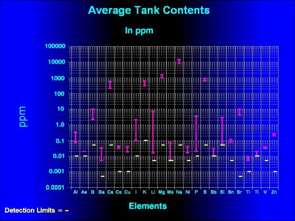Figure 1. Average tank concentrations of those elements whose concentrations were above the detection limits of the test procedure.

In the examinations of Figures 1 and 2, it is important to realize that the horizontal lines represent different things. In Figure 1, the values represent the actual concentrations of the material in ppm, whereas in Figure 2 they represent relative values compared to normal. So, in Figure 2, that a value of "1.00" from the tests indicates an average proportion in the tested tanks that is the same as the average NSW concentration. Similarly, a value crossing the line for "0.1" means the tested value was one tenth the value of the average NSW concentration and a value crossing the line for "100" is one hundred times the NSW value. In Figure 1, these values represent the actual concentrations. Additionally, if you evaluate the differences between the graphs illustrating last month's article and this one, it is important to realize that the observed changes do not reflect any change in the actual values found in the aquaria, but simply are a result of changes in the accepted values in the NSW concentrations.

Prior to trying to assess why the trace element concentrations in these tanks are different from those in NSW, it is also important to consider how we perceive them as different. The samples for these studies were evaluated by one analytical method. Another methodology might give somewhat different results. The methodology used by the lab I chose is called "Inductively Coupled Plasma Emission Spectroscopy." The methodology is reasonably sensitive and may be used for assessing a large number of elements. It is commonly used in environmental testing and assessment, and is relatively inexpensive, as each sample costs less than $200 to process. However, as in all methodologies, there were trade offs. In this case, the trade off came in the assessment of several elements where the detection limits of the test are above the levels commonly found in NSW.

Although the samples were analyzed for Beryllium, Chromium, Cadmium, Iron, Lead, Manganese, Mercury, Selenium, Silver, and Yttrium, none of these elements were detected in the samples; at least in part because the tests simply were not sensitive enough to detect them at normal and near normal concentrations. Most of these elements are quite toxic to marine organisms, but are normally found in very low concentrations and are probably of no consequence to aquarists. Iron and Manganese, however, are biologically active and important for many organisms, and it would have been preferable to have some idea of their concentrations. Nonetheless, neither of these elements was detected in any of the samples. It is important to note, this lack of detection does not mean that the materials were absent, just that the test could not detect them. Those elements will not be discussed further.

In some other cases, as illustrated by Iodide and Tin, where the detection limit for the test is above the NSW concentrations, the aquarium levels detected were all so significantly elevated over the normal NSW levels that the test was able to detect them without a problem. For example, the detection limit for Tin was on the order of 10,500 times greater than the normal level found in sea water. However, the tank concentrations for tin averaged a whopping 200,000 times the level in sea water, so the test had plenty of latitude in which to work (Figure 2).

Iodine presents a special case. Although the initial documentation from the lab indicated that the test was for Iodide ion, a discussion with the laboratory director indicated that the procedure tests for total Iodine, not just Iodide ion. Even though the detection limit for the test was above the NSW level of Iodide, it was below that for total Iodine and well below the tank levels for this material. This was another case where both the upper and lower limits of the tank concentrations were well above both the detection limits and the NSW concentrations.

After examination of these data, questions should arise as to their significance. In effect, what can we learn from such data? Several trace elements are found in elevated concentrations in aquarium water (Table 2; Figure 2). Some of these metals have extremely high concentrations relative to NSW; tin has already been mentioned as having concentrations over 200,000 times above normal, but Thallium, Titanium, Aluminum, Zinc, Cobalt, Antimony, and Copper all have concentrations of over 95 times normal. Conversely, of the detected elements, relatively few are substantially lower than normal. Although Sulfur, Boron, Strontium, Silicon and Vanadium had lower tank concentrations than in NSW, only Vanadium was present at less than about 50 % of normal levels.

In the remainder of this article, I will examine the abundance patterns of the detected chemicals, as well as some other factors, and try to determine if there is any easily evident reason for such patterns. Furthermore, I will try to assess the significance of such patterns and associations.

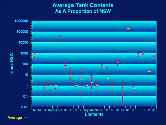Figure 2. Average tank concentrations of the tested elements as a proportion of their concentrations in NSW. Note the vertical scale is logarithmic with each major horizontal line being ten times the value of the one below it.

Materials and Methods

The data from this study are in the form of several independent single samples. As such, the data do not consist of replicate samples of a single treatment, and they can not be easily tested statistically to determine the significance of variations. However, I should point out that such tests were never anticipated, nor planned for. Rather, this was to be a descriptive study of several aquaria to allow the description of "an average reef tank." Within the purview of descriptive statistical analyses is a relatively powerful tool: correlation analysis. This is an analytical procedure using assumptions of a normal distribution. I am not testing for such normality; instead I am assuming it. All of the samples were taken from systems that were being maintained with the explicit goal of maintaining coral reef animal life, and most marine life has relatively low tolerance for variation, it follows that the samples are likely either normally distributed or close enough to normality that the differences from normality should be minor.

Five different categories were simultaneously compared in a single correlation analysis (Table 3). Those items with numerical values, such as concentrations or physical measurements were compared using those measurements. Other measurements, such as the use of RO/DI water, or additives, were entered into the correlation table with values of 1 (= yes) or 0 (= no). There were a total of 44 factors, arrayed over 25 tanks. In the analysis, each factor is compared with every factor, including itself. The resulting matrix, with 44 factors in rows and columns, contained 1936 separate cells, each with a comparison of the row factor with the column factor. Of these, 44 were correlations of the factor with itself. These values are routinely discarded. The remaining matrix, containing 1892 values, contains two identical, but reciprocal parts; for example, for every comparison of A with B, there is a complimentary comparison of B with A. Consequently, there were only 946 different correlation values to examine. Some of these are trivial comparisons, such as when only one category or value is found. Only one of the examined reef tanks used filtered NSW as its water. Thus, each correlation with NSW concerns only one datum per category, and as such has little predictive potential. Similarly, Arsenic was detected in only one tank, so all correlations with arsenic concern only the one tank. Such one-factor correlations have little or no information of value and were not considered further.

The correlation statistic may range from -1.000 to + 1.000. A correlation of 1.00 means the association always occurs and is therefore completely predictable; however, it may be either a positive predictor or a negative one. A correlation value of 0.000 indicates no correlation or predictive value. There is no standard approach to interpreting correlation data; it depends on the data being examined. For the purpose of this study, I define the correlations of 0.500 to 0.650 as weak, those of 0.651 to 0.850 as moderate, and those of 0.851 to 1.000 as strong. Such correlations may be either positive or negative.
The correlation matrix was examined and the values within the range of -0.499 to 0.499 were discarded and all others were classified according to the above criteria.

It is important to remember that CORRELATIONS CANNOT BE USED TO IMPLY CAUSATION. Correlations may be used to infer some causal action, but such a cause needs to be experimentally, or observationally, validated. It is all too easy to examine correlative data and to imply that since factor A and factor B are correlated, they must somehow be reacting or behaving similarly due to some common cause. This is definitely NOT true. We may infer a cause, but without other evidence, such a causal relationship is purely speculative. As I have no experimental data to work with, I will speculate a lot in the discussion portion of this report.

In an attempt to assess potential utilization of materials, I compared the average values found in these tanks with the average values of trace metals in sea water mixes using the data from Atkinson and Bingman (1999) study of artificial sea water mixes.

Results

The correlation values showing associations are shown in Table 4. Relatively few negative correlations were found altogether, although some of them are interesting, such as the negative association of Iodine concentration with Calcium additions, and the negative relationship of Calcium concentration and sand bed depth.

One of the reasons that some of the data appear to be low may be an artifact of data manipulation. The data were adjusted for differences in salinity by normalizing the data as described in Shimek, 2002. If that were the case, one would expect many of these elements with low readings to have the same patterns of abundance. In other words they would show correlations due to the normalization procedure. That is apparently not the case. Sulfur and Boron do have a slight positive association, 0.398, but it is still a weak association at best, and probably indicates little of importance. It, however, is the largest of the correlations concerning the elements with low concentrations. Such weak associations may simply reflect their similar patterns of low abundances in some of salt mixes.

The only strong correlations were all positive ones, and with the exception of the strong correlation between Iodine and Phosphorus, all of them concern Cobalt, Tin, Zinc, Titanium, and Copper. Vanadium is moderately correlated with these metals as well, and it is evident that they form an assemblage of metals which all show similar patterns of distribution and variation (Table 4). Moderate and weak correlations are numerous and some of them are quite interesting; negative correlations are few. The only negative moderate correlation is between Aluminum and Calcium, indicating tanks with high Calcium concentrations tend to have low Aluminum concentrations. Similarly, Aluminum and Strontium are also weakly and negatively correlated with each other, and Strontium is negatively correlated with a number of metals. The weak and moderate positive correlations also indicate that many of the trace metals listed above are correlated with other metals such as Nickel, Zinc, Aluminum and some others.

The most interesting moderate correlations, in my opinion, however, are those involving comparisons with tank factors other than trace elements (Table 5). For example, several metals are correlated with the presence of dissolved fats in the water; additionally, the fat concentrations tend to be higher in older tanks. Tanks which have been set up longer also have high concentrations of nitrogenous compounds. As we will see in the discussions, some of the comparisons may say more about the aquarists than the tanks.

Only 15 trace elements, Aluminum, Barium, Chromium, Cobalt, Copper, Iron, Lead, Lithium, Manganese, Molybdenum, Nickel, Silver, Titanium, Vanadium and Zinc, were examined by both the Atkinson-Bingman (1999) sea water study and this study. One sample in this study was Instant Ocean water, made up with RO/DI , and the values for the trace metals in that sample are quite close to the averages of the salt waters from the Atkinson and Bingman (1999) study. All but Zinc showed lower values in the tanks than in the mixes (Table 6) or the Instant Ocean Sample.

Discussion

The first article of this series detailed an average reef aquarium as described from this sample of 23 tanks (Shimek, 2002). Hidden inside the average values discussed in that article are tendencies within various components of the data to vary in consistent ways. These trends become apparent with the examination of correlative data, for such examinations allow the determination of similar patterns of change that occur within the factors across all the samples. In a very real sense, a correlation coefficient is a statistic describing "trendiness." If two factors have a strong correlation, they are consistently varying in the same manner. Consequently, we can say that if X, Y, and Z are correlated in our aquaria, then tanks with a high concentration of X are likely to have high concentrations of Y and Z as well. Knowing how things change together, and which things change together, is the first step in really understanding what is occurring in our tanks.

We have been able to guess, speculate, and pontificate to our heart's content about how the various factors that are important in the lives of our reef animals change; for example, as tanks age or as we go from a smaller tank to a larger one, but this study allows us for the first time, to get some actual quantitative data to discuss. Additionally, we now have analytical data that allow us to compare 23 tanks in detail.

The examination of the correlations allows us the opportunity to get a feel for the factors and processes occurring in reef tanks. The systems in this study ranged in size from 36 to 380 gallons, and in age from a few weeks to about 10 years (Shimek, 2002). The use of correlative data can allow us to examine trends across both size and age of reef systems, as well as between users of various water types and salts..

A few of the findings are somewhat surprising. Across the size range of these tanks, there were no significant correlations with tank size. This means that for the purposes of describing a reef aquarium with regard to the factors tested in this study, a 35 gallon tank is as good as one of 300 gallons. Although none of these tanks were "nano" reefs, within the size range of normal reef tanks, the systems were all comparable, with no combination of chemicals or tested factors peculiar to either larger or smaller tanks.

Several of the trace metals varied in concert, particularly Cobalt, Tin, Zinc, Titanium, Copper and Vanadium, and lower but still positive correlations with Nickel and Aluminum are found. All of these metals are found at concentrations far above those of natural sea water. Some of these concentrations are almost unbelievably high. Tin has an average concentration in our systems of over 200,000 times greater than in natural sea water. At the same time, it must be pointed out that its average concentration is still low; however, its natural concentration is very much lower. The action of some of these metals in reef animals is not known, for example, it appears quite likely that Titanium may have no effect on reef animals one way or another. On the other hand, some of these metals do have effects. Cobalt is a required co-factor in all aerobic respiration as it is part of Vitamin B12. Copper is also an essential and necessary element for many animals' metabolism; however for many of those same animals, and others, it is quite toxic at very low levels just above their needed concentrations. Vanadium is also very toxic and few marine animals can tolerate it at all. Among those that can metabolize Vanadium are sea squirts, or tunicates, and they use it as an antifouling agent to kill or deter the growth of nearby organisms or organisms that might overgrow them (Figure 3).

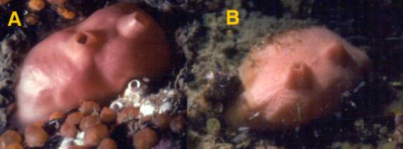Figure 3. Cnemidocarpa finmarkiensis, a temperate sea squirt, each animal is about 1 inch (2.5 cm) long.. The animal in A is healthy: note the body is shiny and devoid of animal and algal growth. Cnemidocarpa and other tunicates secrete Vanadium and other heavy metals through their tunic to kill over-growing or fouling organisms. The animal in B is unhealthy and for some reason appears unable to secrete its antifouling chemicals. Note the overgrowth at the top of brownish algae and at the bottom of whitish hydroids.

Increases in many of these same metals are correlated with the age of the tank. One explanation for that pattern would be that they may build up with the passage of time. The same metals are also correlated with the presence of fat in the aquarium water. It is possible that such fat is related to the types of food given to the aquarium, and that will be reported on next month. If that is the case, the metals' concentrations may simply be related to feeding and foods. It is also possible that the fat in tank water comes from the organisms growing in the system, and as older tanks often have more and larger animals, they would produce more fats. One intriguing possibility is that organisms in the system may secrete the toxic metals as part of their suite of anti-predator and anti-competitor chemicals. No matter what the cause, the build up of such chemicals is a cause for concern.

The older tanks also have more ammonia, nitrate/nitrite, phosphorus, iodine and copper than younger tanks. Nitrate and nitrite are produced either from the decomposition of excess food, which might be present in greater amounts in older tanks, or by the processing of animal urine which is mostly ammonia. The processed urine found in vertebrates, mollusks, and arthropods will also contain Ammonia, Phosphorus and Amino Acids, so it is likely the high levels of these compounds simply reflect more living tissue in older tanks. The higher Iodine levels in older tanks most likely reflect an accumulation, either from feeding or from additives. Tank Iodine concentrations average about 10 times NSW levels. This biologically active element is most frequently found in algal metabolites in marine ecosystems, and its high concentration in the tanks may simply indicate either algal growth or the addition of algal foods and additives. Iodine is also a toxic material when found in high concentrations, and levels such as these may be cause for some concern. Interestingly enough tank iodine concentrations show a slight negative correlation (-0.179) with the use of Iodine additives. The magnitude of this coefficient implies that there is no correlation between the use of Iodine additives and the final tank concentration of this material. Probably much more Iodine is added in the foods, but those data will be investigated next month. The various forms of Iodine vary in biological activity and toxicity. For the present, and with these data, we have no way of estimating their various contributions, either positive or negative to the system.

Additionally, given the logistics of the situation, it was impossible to provide a way to reliably filter the water samples at the time of collection. From the aspects of organisms such as corals, particulates are as much a part of the water environment as are dissolved materials. These small particulates were not filtered prior to analysis, and in all of the samples there are likely varying amounts of particulate organic material. Such material could be responsible for some of the correlative data between Ammonia, Phosphorus, and Amino Acids, and Fat. Also the correlation of Fats with the age of the tank, and some other factors relating indirectly to tank age, may simply reflect the ability of older, more "mature," tanks to generate more living particulate material , either as zooplankton, phytoplankton or bacterioplankton. I feel that the abundance of such plankton is relatively low in most of our systems, but I certainly may be error. Filtering out particulate material prior to the test would have, in my opinion, removed data reflecting total abundances of several elements and was not desirable.

Some of the correlations may tell us more about the aquarists than the aquariums, per se. For example, Titanium grounding probes are negatively correlated with older tanks; this means they are likely to be found in newer tanks. The probes are correlated with tanks that have regular additions of additives. Consequently, it is likely that this means that the newer tanks are maintained by aquarists that think that grounding probes and additives are important. Also, Copper levels are correlated with the use of tap water as a source for mixing the salt water used in the tanks. This Copper likely is related to Copper plumbing, which would be removed in RO/DI water. The plumbing in our houses likely contributes to some of the other metals concentrations as well; as other metals may leach out of solders, or fixtures. The elevated levels of Zinc may be indicative of brass fittings in the plumbing, perhaps some distance upstream of the tap. As a general rule, it may well be a good idea for aquarists who do not use RO/DI water to consider some auxiliary means of removing Copper, Zinc, or other metals.

There were some odd findings. Sand bed depth was weakly, but negatively correlated with both Calcium concentrations and Calcium additives, and positively correlated with Magnesium concentrations, possibly indicating a certain "sloppiness" in the efforts to maintain Calcium by aquarists having deep sand beds.

Additionally, as a series of averages, many of the trace element concentrations are lower than they are in freshly made up artificial sea water. Whether this indicates organism use, or abiotic chemical reactions is unclear. Even though these levels are lower than in "fresh" artificial sea water, they are still very much higher than in natural sea water, and may still indicate a cause for concern.

These patterns are interesting and possibly dependent on several factors. There is likely no single cause for some of the effects, and it is just as likely that there is no defined cause at all for some of them. In these latter cases, the patterns would be the result of random factors or happenstance. The high metals concentrations may be due to build up in the tanks from foods, or from salt formulations, or from the ill-conceived use of poorly formulated additives. Other high concentrations, such as the fats and other metabolites, may be due directly to in-tank metabolism or be caused from food additions. Obviously, aquarist whim and preference may be a major determinant of many of the factors such as iodine and calcium concentrations. Unfortunately without experimentation, we cannot determine causation, and such experimentation would be expensive and time consuming.

For the moment, we are left with some correlations to ponder. Next month, I will discuss the composition of the various foods added to the tanks in this study. From knowing what goes into these systems, and what is there, I will try to estimate some of the materials flow that must be occurring in the systems, and some of the consequences of that flow and the feeding

Acknowledgements:

This article benefited significantly from reviews by Skip Attix, Eric Borneman and Randy Holmes-Farley, and I thank them all for their efforts. Additionally, I would again like to thank the participants and donors who made the Tank Water Study possible: Mark Boenisch, Eric Borneman, Cliff Carter, David Celentano, Allen Chantelois, Steven Collins, Gregory Dawson, John Delery, Adrian Harris, Deborah Lang, Matthew Mengerink, Steven Miller, Steven Nichols, John Link, Jaroslaw Pillardy, Robert Schnell, Sandra Shoup, William Wiley and Anonymous Contributors for contributing water samples. I also thank Danmhippo@reefs.org, Matthew Hennek, Matthew Davis, and Win Phinyawatana for providing cash donations to support this venture. Without all of your assistance, this project would not have been possible.

References Cited:

Atkinson, M. and C. Bingman. 1999. The Composition of Several Synthetic Seawater Mixes. March 1999 Aquarium Frontiers On-line.

Pilson, M. E. Q. 1998. An Introduction to the Chemistry of the Sea. Prentice-Hall, Inc. Upper Saddle River, NJ. 431 pp.

Shimek, R. L. 2002. It's (In) The Water. Reefkeeping.Com. Volume 1. Number 1. February, 2002.

Weast, R. C. 1966. Ed. The Handbook of Chemistry and Physics. 46th edition. Chemical Rubber Company. Cleveland, Ohio. Page F-110.